Data types and classes

STA 199

Bulletin

this ae is due for grade (48 hours from class). To turn in, simply push to GitHub
homework 01 due today at 5:00pm

Getting started

Clone your ae7-username repo from the GitHub organization.

Today

By the end of today you will…

learn how to check the type of a variable
utilize factors

Load packages

We will use the following two packages in this application exercise.

tidyverse: For data import, wrangling, and visualization.
scales: For better axis labels.

library(tidyverse)
library(scales)

Notes

A type is how an object is stored in memory. In this course we’ll encounter the following types:

numeric types:
- double: a real number stored in double-precision floating point format
- integer
character strings
logical (TRUE/FALSE)
lists (a heterogeneous collection of the above)
NULL

Some objects have additional metadata associated with them, called a class. One popular example of a class is a factor. R stores categorical variables as factors.

Example factor

x = factor(c("Monday", "Friday", "Wednesday"))
str(x) # look at the structure of x

 Factor w/ 3 levels "Friday","Monday",..: 2 1 3

attributes(x) # see metadata

$levels
[1] "Friday"    "Monday"    "Wednesday"

$class
[1] "factor"

levels(x) # look at levels of a factor

[1] "Friday"    "Monday"    "Wednesday"

The levels of a factor default to alphabetical order but you can change the order of the levels:

levels(x) = c("Monday", "Wednesday", "Friday")
levels(x)

[1] "Monday"    "Wednesday" "Friday"

Type coercion

Demo: Determine the type of the following vector. And then, change the type to numeric.
```
x = c("1", "2", "3")
typeof(x)
```
```
[1] "character"
```
```
as.numeric(x)
```
```
[1] 1 2 3
```
Demo: Once again, determine the type of the following vector. And then, change the type to numeric. What’s different than the previous exercise?
```
y = c("a", "b", "c")

# add code here
```
Demo: Once again, determine the type of the following vector. And then, change the type to numeric. What’s different than the previous exercise?
```
z = c("1", "2", "three")

# add code here
```
Demo: Suppose you conducted a survey where you asked people how many cars their household owns collectively. And the answers are as follows:

survey_results = tibble(cars = c(1, 2, "three"))
survey_results

# A tibble: 3 × 1
  cars 
  <chr>
1 1    
2 2    
3 three

This is annoying because of that third survey taker types a character string instead of providing a numeric value. So now you need to update the cars variable to be numeric. You do the following

survey_results |>
mutate(cars = as.numeric(cars))

Warning in mask$eval_all_mutate(quo): NAs introduced by coercion

# A tibble: 3 × 1
   cars
  <dbl>
1     1
2     2
3    NA

Now you get a warning NAs introduced by coercion that happened while computing cars = as.numeric(cars) and the response from the third survey taker is now an NA (you lost their data). Fix your mutate() call to avoid this warning.

survey_results |>
  mutate(cars = if_else(cars == "three", "3", cars),
         cars = as.numeric(cars))

# A tibble: 3 × 1
   cars
  <dbl>
1     1
2     2
3     3

Exercise 1

First, guess the type of the vector. Then, check if you guessed right. I’ve done the first one for you, you’ll see that it’s helpful to check the type of each element of the vector first.

c(1, 1L, "C")

v1 = c(1, 1L, "C")

# to help you guess
typeof(1)

[1] "double"

typeof(1L)

[1] "integer"

typeof("C")

[1] "character"

# to check after you guess
typeof(v1)

[1] "character"

v2 = c(1L / 0, "A")

-   `c(1:3, 5)`

v3 = c(1:3, 5)

-   `c(3, "3+")`

v4 = c(3, "3+")

-   `c(NA, TRUE)`

v5 = c(NA, TRUE)

Useful coercion

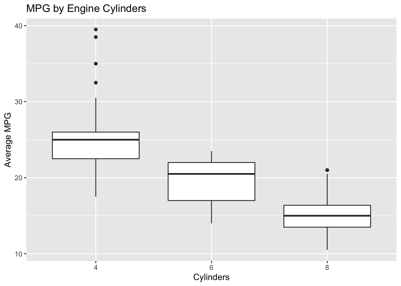
Exercise 2

data(mpg)

Recreate the plot below. Make sure axes and title labels are exactly matching, including spelling, capitalization, etc.

Hint

You will need to use as.factor() to cast the appropriate variable as a factor.

# code here

Hotel bookings

# From TidyTuesday: https://github.com/rfordatascience/tidytuesday/blob/master/data/2020/2020-02-11/readme.md

hotels = read_csv("https://raw.githubusercontent.com/rfordatascience/tidytuesday/master/data/2020/2020-02-11/hotels.csv")

Exercise 3

Take a look at the the following visualization. How are the months ordered? What would be a better order?

Reorder the months on the x-axis (levels of arrival_date_month) in a way that makes more sense. Use the factor() function to mutate the column into a factor. Read ?factor for help.

hotels |>
  group_by(hotel, arrival_date_month) |>   # group by hotel type and arrival month
  summarise(mean_adr = mean(adr), .groups = "drop") |>       # calculate mean adr for each group
  ggplot(aes(
    x = arrival_date_month,                 # x-axis = arrival_date_month
    y = mean_adr,                           # y-axis = mean_adr calculated above
    group = hotel,                          # group lines by hotel type
    color = hotel)                          # and color by hotel type
  ) +
  geom_line() +                             # use lines to represent data
  theme_minimal() +                         # use a minimal theme
  labs(
    x = "Arrival month",                 # customize labels
    y = "Mean ADR (average daily rate)",
    title = "Comparison of resort and city hotel prices across months",
    subtitle = "Resort hotel prices soar in the summer while ciry hotel prices remain relatively constant throughout the year",
    color = "Hotel type"
  )

Optional extra: Change the y-axis label so the values are shown with dollar signs, e.g. $80 instead of 80. You will want to use a function from the scales package, see https://scales.r-lib.org/reference/index.html for inspiration and help.