Spatial data

STA 199

Bulletin

this ae is due for grade (48 hours from class). To turn in, simply push to GitHub
check your ae grades in Sakai
lab-3 due Friday at 5:00pm
exam 1 released Friday at 5:00pm
find solutions to the practice, labs and aes on Sakai under resources tab

Getting started

Clone your ae8-username repo from the GitHub organization.

Today

By the end of today you will…

understand spatial data frame structure
be able to create a visualization from a spatial data frame

Load packages

library(tidyverse)
library(sf)

Notes

Spatial data is different.

Our typical “tidy” dataframe.

mpg

# A tibble: 234 × 11
   manufacturer model      displ  year   cyl trans drv     cty   hwy fl    class
   <chr>        <chr>      <dbl> <int> <int> <chr> <chr> <int> <int> <chr> <chr>
 1 audi         a4           1.8  1999     4 auto… f        18    29 p     comp…
 2 audi         a4           1.8  1999     4 manu… f        21    29 p     comp…
 3 audi         a4           2    2008     4 manu… f        20    31 p     comp…
 4 audi         a4           2    2008     4 auto… f        21    30 p     comp…
 5 audi         a4           2.8  1999     6 auto… f        16    26 p     comp…
 6 audi         a4           2.8  1999     6 manu… f        18    26 p     comp…
 7 audi         a4           3.1  2008     6 auto… f        18    27 p     comp…
 8 audi         a4 quattro   1.8  1999     4 manu… 4        18    26 p     comp…
 9 audi         a4 quattro   1.8  1999     4 auto… 4        16    25 p     comp…
10 audi         a4 quattro   2    2008     4 manu… 4        20    28 p     comp…
# … with 224 more rows

A new simple feature object.

nc <- st_read("data/nc_regvoters.shp", quiet = TRUE)
nc

Simple feature collection with 100 features and 8 fields
Geometry type: MULTIPOLYGON
Dimension:     XY
Bounding box:  xmin: -84.32385 ymin: 33.88199 xmax: -75.45698 ymax: 36.58965
Geodetic CRS:  NAD27
First 10 features:
      county   dem   rep lib  unaf  male female  total
1   ALAMANCE 38209 35967 670 35196 44651  54529 110042
2  ALEXANDER  4772 11750 123  7967 10947  11768  24612
3  ALLEGHANY  2030  3005  33  2466  3319   3548   7534
4      ANSON  9130  2858  38  3599  5800   6980  15625
5       ASHE  4261  8804 102  6232  8609   9525  19399
6      AVERY  1343  6994  55  3673  5283   5829  12065
7   BEAUFORT 10883 11873 124  9426 13591  16127  32306
8     BERTIE  8178  1629  36  2835  5310   6610  12678
9     BLADEN  9847  5005  77  6784  9472  11227  21713
10 BRUNSWICK 26797 46557 618 42602 48199  55644 116574
                         geometry
1  MULTIPOLYGON (((-79.24619 3...
2  MULTIPOLYGON (((-81.10889 3...
3  MULTIPOLYGON (((-81.23989 3...
4  MULTIPOLYGON (((-79.91995 3...
5  MULTIPOLYGON (((-81.47276 3...
6  MULTIPOLYGON (((-81.94135 3...
7  MULTIPOLYGON (((-77.10377 3...
8  MULTIPOLYGON (((-76.78307 3...
9  MULTIPOLYGON (((-78.2615 34...
10 MULTIPOLYGON (((-78.65572 3...

Exercise 1

What differences do you observe when comparing a typical tidy data frame to the new simple feature object?

Simple features

A simple feature is a standard, formal way to describe how real-world spatial objects (country, building, tree, road, etc) can be represented by a computer.

The package sf implements simple features and other spatial functionality using tidy principles. Simple features have a geometry type. Common choices are shown in the slides associated with today’s lecture.

Simple features are stored in a data frame, with the geographic information in a column called geometry. Simple features can contain both spatial and non-spatial data.

All functions in the sf package helpfully begin st_.

`sf` and `ggplot`

To read simple features from a file or database use the function st_read().

nc <- st_read("data/nc_regvoters.shp", quiet = TRUE)

Notice nc contains both spatial and nonspatial information.

We can build up a visualization layer-by-layer beginning with ggplot. Let’s start by making a basic plot of North Carolina counties.

nc |>
ggplot() +
  geom_sf() +
  labs(title = "North Carolina counties")

Now adjust the theme with theme_bw().

ggplot(nc) +
  geom_sf() +
  labs(title = "North Carolina counties with theme") + 
  theme_bw()

Now adjust color in geom_sf to change the color of the county borders.

ggplot(nc) +
  geom_sf(color = "darkgreen") +
  labs(title = "North Carolina counties with theme and aesthetics") + 
  theme_bw()

Then increase the width of the county borders using size.

ggplot(nc) +
  geom_sf(color = "darkgreen", size = 1.5) +
  labs(title = "North Carolina counties with theme and aesthetics") +
  theme_bw()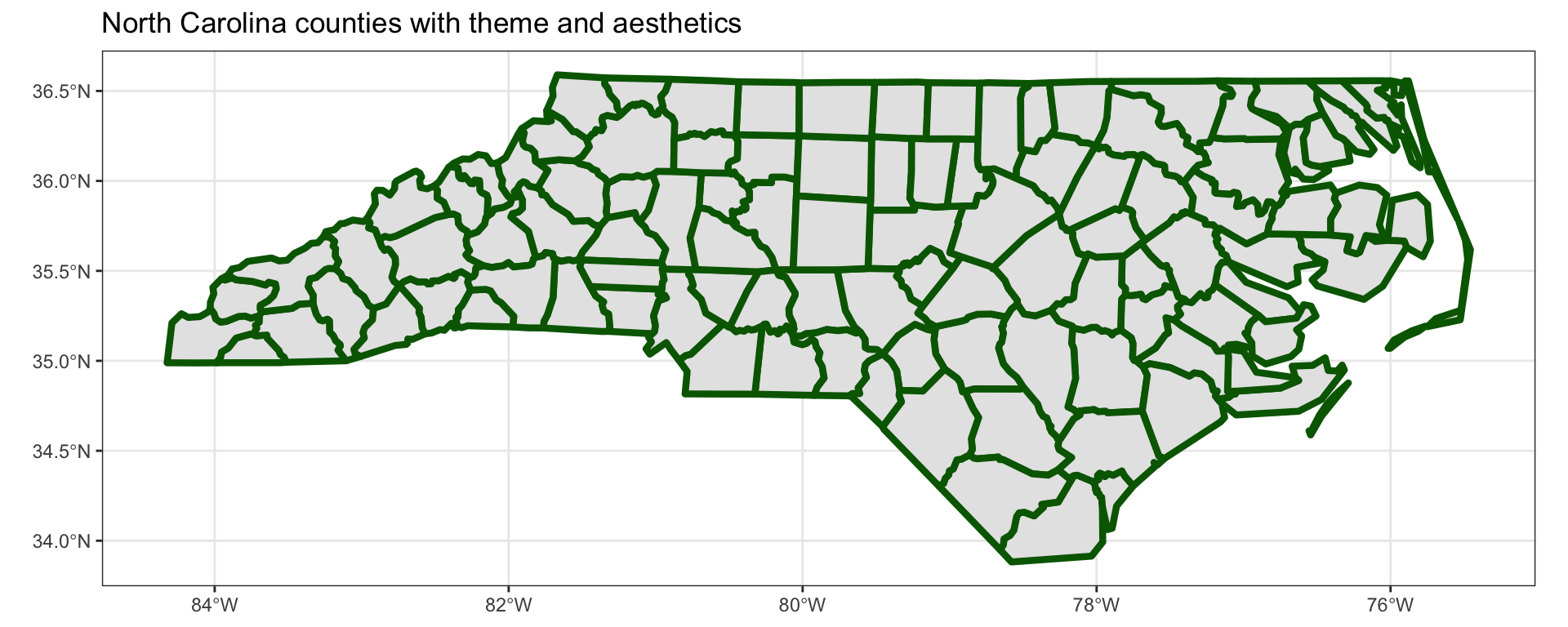

Fill the counties by specifying a fill argument.

ggplot(nc) +
  geom_sf(color = "darkgreen", size = 1.5, fill = "orange") +
  labs(title = "North Carolina counties with theme and aesthetics") +
  theme_bw()

Finally, adjust the transparency using alpha.

ggplot(nc) +
  geom_sf(color = "darkgreen", size = 1.5, fill = "orange", alpha = 0.50) +
  labs(title = "North Carolina counties with theme and aesthetics") +
  theme_bw()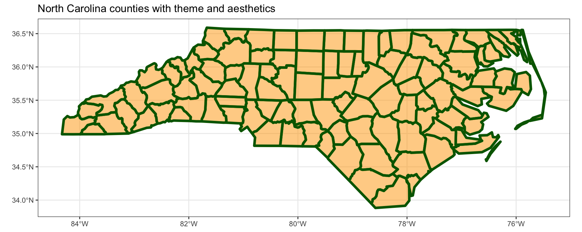

North Carolina Registered Voters

The nc data was obtained from the NC Board of Elections website and contains statistics on NC registered voters as of September 4, 2021.

The data set contains the following variables on all North Carolina counties, categories provided by the NCSBE:

county: county name
dem: total number registered Democrats
rep: total number registered Republicans
lib: total number registered Libertarians
unaf: total number unaffiliated
male: total number male voters
female: total number female voters
total: total number of registered voters in county
geometry: geographic coordinates of the county

Let’s use the NCBSE data to generate a choropleth map of the number of registered voters by county.

ggplot(nc) +
  geom_sf(aes(fill = total)) + 
  labs(title = "Number of Registered Voters by County",
       fill = "# voters") + 
  theme_bw()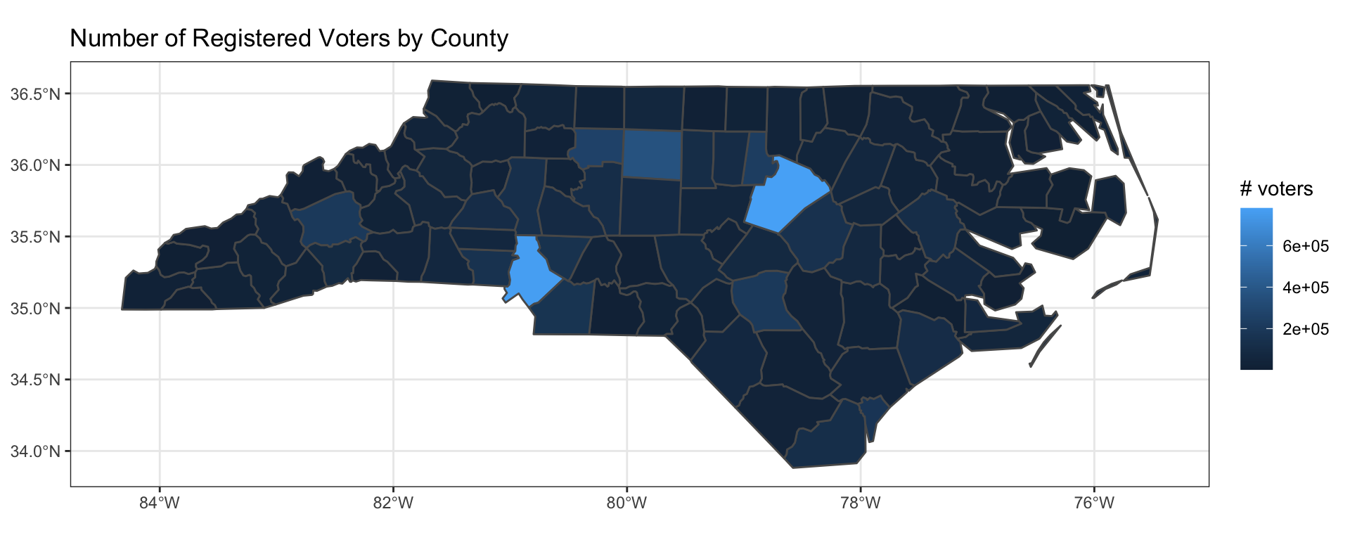

It is sometimes helpful to pick diverging colors, colorbrewer2 can help.

One way to set fill colors is with scale_fill_gradient().

ggplot(nc) +
  geom_sf(aes(fill = total)) +
  scale_fill_gradient(low = "#fee8c8", high = "#7f0000") +
  labs(title = "The Triangle and Charlotte have the Most Voters",
       fill = "# cases") + 
  theme_bw()

Challenges

Different types of data exist (raster and vector).
The coordinate reference system (CRS) matters.
Manipulating spatial data objects is similar, but not identical to manipulating data frames.

`dplyr`

sf objects plays nicely with our earlier data wrangling functions from dplyr.

Example

Maybe you are interested in the percentage of registered democrats/republicans in a county.

nc |>
  mutate(pct_dem = dem / total,
         pct_rep = rep / total) |>
  select(pct_dem, pct_rep)

Simple feature collection with 100 features and 2 fields
Geometry type: MULTIPOLYGON
Dimension:     XY
Bounding box:  xmin: -84.32385 ymin: 33.88199 xmax: -75.45698 ymax: 36.58965
Geodetic CRS:  NAD27
First 10 features:
     pct_dem   pct_rep                       geometry
1  0.3472220 0.3268479 MULTIPOLYGON (((-79.24619 3...
2  0.1938892 0.4774094 MULTIPOLYGON (((-81.10889 3...
3  0.2694452 0.3988585 MULTIPOLYGON (((-81.23989 3...
4  0.5843200 0.1829120 MULTIPOLYGON (((-79.91995 3...
5  0.2196505 0.4538378 MULTIPOLYGON (((-81.47276 3...
6  0.1113137 0.5796933 MULTIPOLYGON (((-81.94135 3...
7  0.3368724 0.3675169 MULTIPOLYGON (((-77.10377 3...
8  0.6450544 0.1284903 MULTIPOLYGON (((-76.78307 3...
9  0.4535071 0.2305071 MULTIPOLYGON (((-78.2615 34...
10 0.2298712 0.3993772 MULTIPOLYGON (((-78.65572 3...

Geometries are “sticky”. They are kept until deliberately dropped using st_drop_geometry.

nc |> 
  select(county, total) |> 
  st_drop_geometry()

          county  total
1       ALAMANCE 110042
2      ALEXANDER  24612
3      ALLEGHANY   7534
4          ANSON  15625
5           ASHE  19399
6          AVERY  12065
7       BEAUFORT  32306
8         BERTIE  12678
9         BLADEN  21713
10     BRUNSWICK 116574
11      BUNCOMBE 201401
12         BURKE  57481
13      CABARRUS 148489
14      CALDWELL  53537
15        CAMDEN   7646
16      CARTERET  52097
17       CASWELL  15195
18       CATAWBA 107060
19       CHATHAM  57602
20      CHEROKEE  22010
21        CHOWAN   9685
22          CLAY   9129
23     CLEVELAND  66186
24      COLUMBUS  35646
25        CRAVEN  68989
26    CUMBERLAND 201336
27     CURRITUCK  21189
28          DARE  30151
29      DAVIDSON 111819
30         DAVIE  31265
31        DUPLIN  30586
32        DURHAM 228967
33     EDGECOMBE  33798
34       FORSYTH 263103
35      FRANKLIN  47475
36        GASTON 150351
37         GATES   8050
38        GRAHAM   5944
39     GRANVILLE  39468
40        GREENE  10565
41      GUILFORD 366867
42       HALIFAX  36047
43       HARNETT  79170
44       HAYWOOD  45241
45     HENDERSON  85808
46      HERTFORD  14308
47          HOKE  32002
48          HYDE   3003
49       IREDELL 129972
50       JACKSON  28551
51      JOHNSTON 144074
52         JONES   6826
53           LEE  37792
54        LENOIR  35854
55       LINCOLN  63412
56         MACON  26868
57       MADISON  16636
58        MARTIN  15977
59      MCDOWELL  29049
60   MECKLENBURG 773683
61      MITCHELL  11004
62    MONTGOMERY  16821
63         MOORE  72611
64          NASH  66185
65   NEW HANOVER 172138
66   NORTHAMPTON  13139
67        ONSLOW 107577
68        ORANGE 105638
69       PAMLICO   9157
70    PASQUOTANK  27127
71        PENDER  45024
72    PERQUIMANS   9813
73        PERSON  27017
74          PITT 113718
75          POLK  15772
76      RANDOLPH  93805
77      RICHMOND  27216
78       ROBESON  69785
79    ROCKINGHAM  60497
80         ROWAN  95376
81    RUTHERFORD  45278
82       SAMPSON  37263
83      SCOTLAND  20153
84        STANLY  42752
85        STOKES  31547
86         SURRY  46850
87         SWAIN   9774
88  TRANSYLVANIA  25854
89       TYRRELL   2268
90         UNION 161006
91         VANCE  28412
92          WAKE 780519
93        WARREN  12940
94    WASHINGTON   8050
95       WATAUGA  43127
96         WAYNE  73786
97        WILKES  43527
98        WILSON  54424
99        YADKIN  24494
100       YANCEY  14197

Exercise 2

Construct an effective visualization investigating the per county percentage of unaffiliated voters in NC. Use #f7fbff as “low” on the color gradient and #08306b as “high”. Which county has the highest percentage of unaffiliated voters? (You might want to use Google here.)

# code here

Write a brief research question that you could answer with this data set and then investigate it here.

# code here

What are limitations of your visualizations above?