library(tidyverse)
library(tidymodels)Intro to hypothesis tests
STA 199
Bulletin
- this
aeis due for grade. Push your completed ae to GitHub within 48 hours to receive credit - homework 4 due today
- project draft report due April 7th to your GitHub repo.
Getting started
Clone your ae21-username repo from the GitHub organization.
Today
By the end of today you will…
- Be familiar with the terms “p-value”, “null-distribution”, “null hypothesis”, “alternative hypothesis”
- Compute a p-value
Load packages
Introduction to hypothesis testing
Is this a fair coin?
We’ll record 1 if the coin is “Heads” and 0 if the coin lands “Tails”.
# coin_flips = c()If the coin is fair, what is the probability of seeing the outcome we saw? To answer this question we’ll setup a statistical model:
\[ \text{\# heads} \sim Binomial(n, p) \]
where \(p\) is the probability of a heads and \(n\) is the total number of coin flips.
Exercise 2
If the coin is fair, what would \(p\) be?
Using
R, flip a fair coin 6 times and count the number of heads. Next, repeat this experiment 1000 times and count the proportion of times you observe 6 heads.
# code here- What is the probability of observing 6 heads in 6 coin flips?
Hypothesis testing framework
You may not have realized it but you just performed a hypothesis test!
You setup a null hypothesis: \(H_0\). The null hypothesis is a hypothesis you set up and then try and knock down. Conceptually, it’s the “nothing special is going on” hypothesis. Formally, the null hypothesis makes a claim or assumption about a population parameter.
In this case, it was the assumption that the coin is fair. Mathematically, we write this:
\[ H_0: p = 0.5 \]
Conceptually, \(p\) is the probability of flipping a head if we flipped the coin infinitely many times.
Since we computed the probability of observing all heads, we were fundamentally interested in if \(p > 0.5\). This is our alternative hypothesis, \(H_A\). In mathematical notation, we write
\[ H_A: p > 0.5 \]
Next, we simulated under the null. This means that we simulated what the coin flips would have looked like if the null was true. In this context, this means we simulated as if the coin was fair.
Finally, we check to see where our actual observed data places under the null distribution. If it’s way out in the tail, we reject the null. If its not way out in the tail, we fail to reject the null.
How can we make “way out in the tail” more precise? Well, it’s arbitrary and context-dependent. In some contexts it is popular to use a cut-off of \(0.05\). This cutoff is called “the significance level” and is also known as \(\alpha\).
Exercise 3
Assume we continue flipping our coin for a total of 30 coin flips and observe 23 heads and 7 tails. What is the probability of seeing 23 or more heads if the coin is fair?
# code herep-values
You might not realize it, but you just computed a p-value… again!
A p-value is a probability. It’s the tail probability associated with your alternative hypothesis.
The alternative hypothesis must always relate to the null. Here we had three options:
- \(H_A: p < 0.5\), the coin is biased to land tails
- \(H_A: p > 0.5\), the coin is biased to land heads
- \(H_A: p \neq 0.5\), the coin is biased
Let’s look offline at what each one would like here.
Exercise 4
Compute the p-value associated with each of the alternative hypotheses above.
# code hereMake a conclusion based on a significance level of 0.05. In other words,
- if p < 0.05, reject the null.
- if p > 0.05, we fail to reject the null.
As you can see our conclusion depends on our alternative hypothesis. For this reason, it is important to set up an alternative hypothesis before looking at the data.
Recap
We were interested in whether or not a coin was fair. We let \(p\) be the probability of landing heads. Fundamentally, we were interested in whether or not \(p = 0.5\). This was our null hypothesis:
\[ H_0: p = .5 \]
and our alternative, was that the coin was biased heads:
\[ H_A: p > 0.5 \]
In one example our data consisted of 30 coin flips and 23 heads. The proportion of heads that we observed, \(\hat{p} = 23/30 = .77\).
Do these 30 coin flips give us enough evidence to reject the null in favor of the alternative?
To answer this question, we computed the p-value: \(Pr(\hat{p} \geq .77 | H_0 \text{ true})\). In words, the probability that our statistic of interest, (\(\hat{p}\)), is greater than or equal to what we saw given that the null is true.
Notice that the p-value is defined by three things:
- our observed statistic (0.77)
- the null hypothesis (\(H_0\))
- the alternative hypothesis (\(H_A\)), this tells us the direction (\(>=\)) to shade.
We compared the p-value to some pre-defined cutoff, \(\alpha\). In our example we set our cutoff at \(\alpha = 0.05\). If p-value \(< \alpha\), we reject the null. If p-value \(> \alpha\), we fail to reject the null.
The tidy way
coin_flips = data.frame(one_flip = sample(c(rep("H",23), rep("T", 7)), size = 30))

glimpse(coin_flips)
Rows: 30
Columns: 1
$ one_flip <chr> "H", "H", "H", "H", "T", "H", "T", "H", "H", "H", "T", "H", "…set.seed(2022)
null_dist =
coin_flips %>%
specify(response = one_flip, success = "H") %>%
hypothesize(null = "point", p = 0.5) %>%
generate(reps = 10000, type = "draw") %>%
calculate(stat = "prop")
obs_stat = 23/30
visualize(null_dist) +
shade_p_value(obs_stat, direction = "right")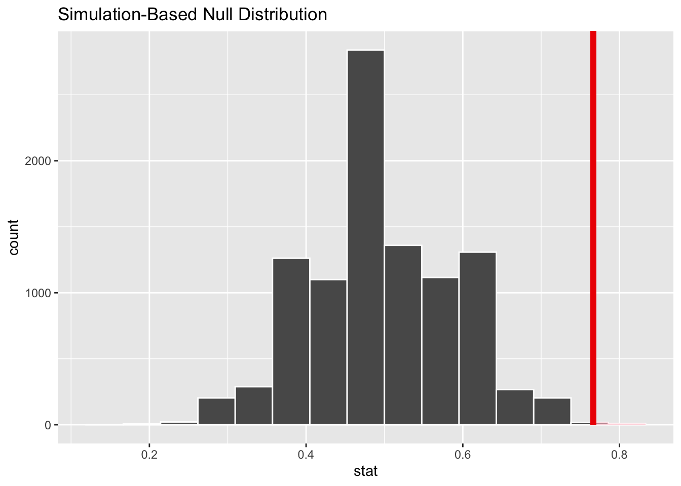
null_dist %>%
get_p_value(obs_stat, direction = "right")
# A tibble: 1 × 1
p_value
<dbl>
1 0.0027p-value of \(0.0027 < 0.05\). We reject the null hypothesis that the coin is fair.